Optimum Pipe Diameter Calculator – Economic Pipe Sizing
The Optimum Pipe Diameter Calculator determines the most economical pipe size for fluid transport systems using the minimum annual cost method. Proper pipe sizing is an important engineering decision because the diameter of a pipe directly affects both the capital cost of installation and the long-term energy cost of pumping.
If the pipe diameter is too small, fluid velocity increases, resulting in larger friction losses and higher pumping power. Conversely, very large pipes reduce friction losses but increase material and installation costs. The optimal design is therefore a balance between capital investment and operating energy cost.
This calculator evaluates hydraulic losses, pump power requirements, and cost scaling relationships to identify the pipe diameter that minimizes the total annual cost of a pumping system.
Effect of Pipe Size on Pumping Cost
Pipe diameter strongly influences the economics of fluid transport systems. The relationship between pipe size and system cost can be summarized as follows:
- Small pipe diameter → high velocity → high friction loss → higher pumping power and energy cost.
- Large pipe diameter → lower friction loss → lower pumping power but higher pipe material and installation cost.
- Optimum diameter → balances capital cost and operating energy cost to achieve the lowest total annual cost.
Economic pipe sizing is widely used in the design of water distribution systems, process pipelines, HVAC circulation loops, and industrial pumping systems.
Traditional Method for Economic Pipe Sizing
Traditionally, engineers determine the optimum pipe diameter through an iterative procedure that involves evaluating multiple candidate pipe sizes. For each pipe diameter, the following steps are performed:
- Calculate fluid velocity and Reynolds number.
- Determine the friction factor and pipe head loss.
- Compute the required pump power.
- Estimate annual energy cost based on electricity price and operating hours.
- Estimate pipe capital cost using empirical cost scaling relationships.
- Convert capital cost into an equivalent annual cost.
- Repeat the calculation for several pipe diameters.
- Select the diameter that produces the lowest total annual cost.
While this method is accurate, performing these calculations manually can be time-consuming and prone to error, particularly when fittings, valves, and economic parameters are included.
Why Use This Calculator?
This calculator automates the hydraulic and economic analysis required to determine the optimum pipe diameter. Instead of performing repetitive manual calculations, engineers can quickly evaluate multiple pipe sizes and identify the economically optimal design.
- Automatic friction loss calculation including fittings and valves
- Built-in pipe roughness database for common materials
- Integrated economic analysis using annual cost methods
- Support for both mass flow rate and volumetric flow rate inputs
- Graphical visualization of capital, energy, and total annual cost
- Identification of the pipe diameter corresponding to minimum cost
The cost curve produced by the calculator visually confirms the diameter that minimizes the total annual system cost.
Steps for Using the Optimum Pipe Diameter Calculator
- Enter the flow rate of the fluid (mass flow or volumetric flow).
- Specify the elevation and pressure profile of the system to determine the required pumping head.
- Input the pipe length and pipe material so that friction losses can be evaluated.
- Enter the economic parameters including electricity cost, operating hours per year, and project life.
- Provide the fluid properties such as density and viscosity.
- Select the pump type and efficiency.
- Include fittings and valves to account for minor losses.
- Click Calculate Optimum Pipe Diameter to determine the pipe size that minimizes total annual cost.
System Inputs
System Schematic
Results
Optimization Result
Energy Balance Terms
Hydraulic Parameters
Optimum Pipe Diameter Calculation Examples (Step-by-Step)
The following worked examples demonstrate how the Optimum Pipe Diameter Calculator can be used to determine the economic pipe size and corresponding pump power requirement for real pumping systems. Each example illustrates the step-by-step procedure for evaluating hydraulic losses, estimating pumping energy consumption, and comparing capital and operating costs in order to identify the pipe diameter that minimizes the total annual cost of the system.
These examples are representative of problems encountered in fluid mechanics, chemical engineering, and mechanical engineering courses as well as practical industrial pumping system design.
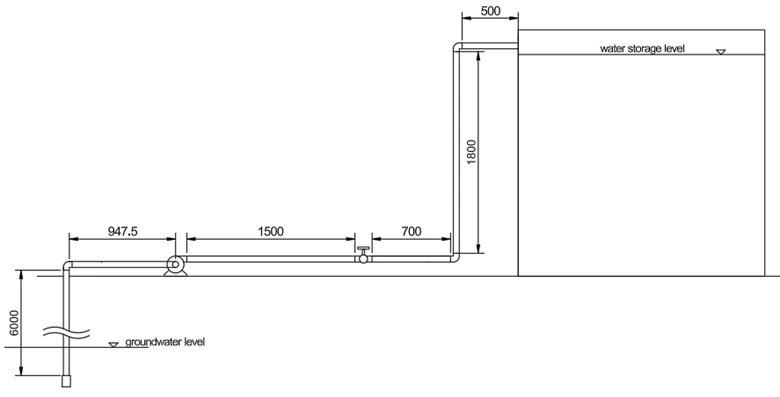
Example 1: Optimum Pipe Diameter for Pumping Groundwater to a Storage Tank
Groundwater at 25 °C is pumped to a storage tank using commercial steel pipes as shown in Figure 1. A gate valve is installed for maintenance purposes and remains fully open during operation. A foot valve is installed at the end of the suction line.
The elevation difference between the groundwater surface and the pipe outlet is 6.8 m. The required flow rate is 100 gallons per minute (gpm). A centrifugal pump with an efficiency of 60% will be used.
Economic parameters are provided to determine the optimum pipe diameter that minimizes the total annual cost of the pumping system.
- Pump service life: 10 years
- Operating hours: 2,190 h/year
- Electricity cost: $0.14/kWh
- Pipe Cost Index: 100
Assumptions
- Dissolved solids in groundwater have negligible effect on water properties.
- Atmospheric pressure difference between inlet and outlet is negligible.
Mechanical Energy Balance Equation
The theoretical pump work is determined using the mechanical energy balance:
Ws = ΔPE + ΔKE + ΔP/ρ + Ftotal
The actual pump power accounts for pump efficiency:
Wa = Ws / η
Economic Analysis
The optimum pipe diameter is determined by minimizing the total annual cost of the system, which consists of energy cost and annualized capital cost.
Total Annual Cost = Annual Energy Cost + Annualized Capital Cost
Annual Energy Cost
Energy cost depends on the pump power, operating time, and electricity price:
Cenergy = Ppump × t × Celectricity
- Pump power = kW
- Operating hours per year = 2190 h
- Electricity cost = $0.14/kWh
Pipe Capital Cost Scaling
Pipe cost typically follows an empirical scaling relationship:
Pipe Cost ∝ D1.8
Fittings and valves scale approximately as:
Fittings Cost ∝ D2
These relationships reflect the increase in material usage and manufacturing complexity as pipe diameter increases.
Use of Pipe Cost Index
Actual piping costs depend on market conditions such as material prices, labor costs, and manufacturing demand. A Pipe Cost Index (PCI) is used to adjust capital cost estimates.
C = Cref (D / Dref)n (PCI / PCIref)
- C = estimated capital cost
- D = candidate pipe diameter
- n = cost exponent (typically 1.8–2.0)
- PCI = current pipe cost index
Simple Annuity Method
Capital cost must be converted into an equivalent annual cost so it can be compared fairly with yearly energy expenses.
Cannual = Ccapital / N
- Cannual = annualized capital cost
- Ccapital = initial pipe cost
- N = project life (years)
For this example:
N = 10 years
Step-by-Step Calculator Procedure
- Input flow rate: 100 gpm
-
Elevation profile
Elevation difference = 6.8 m
Relative elevation = source below discharge
Elevation measured between source liquid surface and pipe outlet -
Pressure profile
Pressure 1 = 100000 Pa
Pressure 2 = 100000 Pa -
Pipe specification
Pipe material: commercial steel
Total pipe length: 11.4475 m -
Economic parameters
- Economic model: Simple Annuity
- Project life: 10 years
- Electricity cost: 0.14 $/kWh
- Operating hours: 2190 h/year
- Pipe cost index: 100
-
Fluid properties
Density = 995.71 kg/m³
Viscosity = 853.83 µPa·s -
Pump selection
Pump type: centrifugal pump
Efficiency: 60% -
Add fittings
- Foot valve (1 pc)
- 90° elbow (3 pcs)
- Gate valve fully open, 100% (1 pc)
- Click Calculate Optimum Pipe Diameter
Note: All fittings and valves added to the system will appear in the fittings list below the schematic. If a component is added incorrectly, it can be removed by clicking the “×” button next to the corresponding fitting or valve.
Results
The calculator predicts an optimum pipe inner diameter of:
2.5 in (63.5 mm)
This corresponds approximately to a 3-inch nominal pipe.
The corresponding actual pump power requirement is:
1.168 kW (1.57 hp)
Comparison with Smaller Pipe
The optimized pipe diameter significantly reduces energy consumption. For comparison, using a 1½-inch Schedule 40 commercial steel pipe in the Pump Power Calculator example results in a pump power requirement of 3.711 kW.
By increasing the pipe diameter to the economically optimal size, the pump power decreases to 1.168 kW, representing a 68.52% reduction in required pump power. This demonstrates how proper pipe sizing can dramatically reduce long-term pumping energy costs.
Energy Balance Terms
| Term | Value | Unit |
|---|---|---|
| Pipe Velocity | 1.9922 | m/s |
| Economic Velocity Range | 1 – 3 | m/s |
| Velocity Assessment | Within economic range | - |
| Total Head Loss | 42.9155 | J/kg |
| Annual Energy Cost | 358.20 | $ |
| Annualized Capital Cost | 595.67 | $ |
| Total Annual Cost | 953.86 | $ |
Hydraulic Parameters
| Parameter | Value | Unit |
|---|---|---|
| Optimum Diameter | 2.5 | in |
| Reynolds Number | 1.475e+5 | - |
| Flow Regime | Turbulent | - |
| Total Loss Coefficient | 21.6270 | - |
Engineering Insight
The calculated pipe velocity is 1.99 m/s, which lies within the typical economic velocity range of 1–3 m/s for water transport systems.
This indicates that the selected pipe diameter provides a good balance between friction losses, pumping power, and pipe capital cost.
Design Note:
The optimum pipe diameter calculated in this analysis represents the economic inner diameter that minimizes the total annual cost of the pumping system.
In practice, pipes are manufactured using nominal pipe sizes (NPS) and specific schedule numbers, which determine the actual inner diameter of the pipe. Therefore, the final pump power requirement should be recalculated using the selected nominal pipe size and schedule number to ensure accurate hydraulic analysis.
You can verify the final pump power requirement using the Pump Power Calculator.
A dedicated Schedule Number Pipe Calculator will also be available on this platform to help determine the actual inner diameter corresponding to each nominal pipe size and schedule number.
Finally, engineers should verify that the pumping system has sufficient Net Positive Suction Head (NPSH) to prevent cavitation. This can be evaluated using the NPSH Available Calculator.
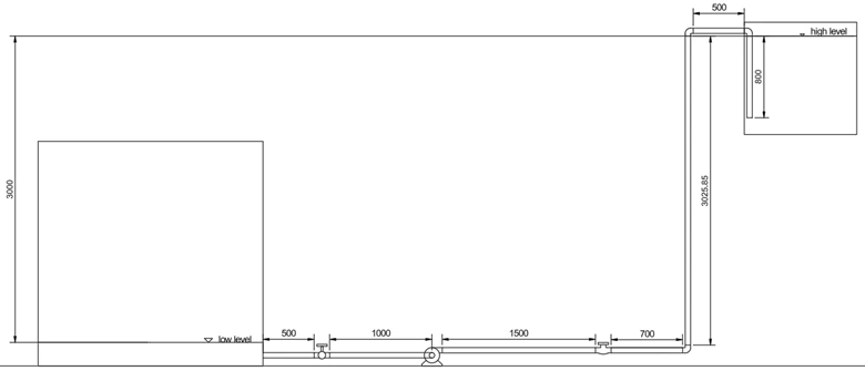
Example 2: Optimum Pipe Diameter for Pumping Molasses Between Tanks
Molasses is pumped from a ground-level storage tank to an elevated receiving tank in a fermentation plant at a rate of 15 m³/h.
Because molasses is highly viscous and susceptible to air entrainment, the discharge pipe is submerged below the liquid level of the receiving tank to minimize splashing and bubble formation.
The fluid is transferred using a rotary lobe pump with an efficiency of 75%. The pipeline consists of commercial steel pipe equipped with a diaphragm valve for isolation and a check valve to prevent backflow.
The maximum elevation difference between the storage tank and receiving tank is 3 m (3000 mm).
Determine the optimum pipe inner diameter for the pipeline if the pumping system operates under the following conditions:
- Project life: 15 years
- Operating time: 3600 hours per year
- Bank lending rate: 8% per year
- Electricity cost: $0.14/kWh
- Pipe Cost Index: 100
Assume atmospheric pressure at both liquid surfaces.
Relevant properties of molasses:
- Density = 1400 kg/m³
- Viscosity = 8 Pa·s
Engineering Approach
This problem is solved using the same hydraulic and economic principles introduced in Example 1. The calculator evaluates different pipe diameters and determines the diameter that minimizes the total annual cost, which includes:
- Annualized capital cost of piping and fittings
- Annual pumping energy cost
In this example, the capital cost is annualized using the Capital Recovery Factor (CRF).
Capital Recovery Factor (CRF)
The Capital Recovery Factor converts a one-time capital investment into an equivalent annual cost while accounting for the time value of money.
CRF Formula:
CRF = i(1+i)n / [(1+i)n − 1]
Where:
- i = annual interest rate
- n = project life (years)
The annualized capital cost is then calculated as:
Annual Capital Cost = Capital Investment × CRF
This method provides a more realistic economic evaluation because it accounts for financing and investment costs.
Step-by-Step Calculator Procedure
- Input flow rate: 15 m³/h
-
Elevation profile
Elevation difference = 3 m
Relative elevation = source above discharge
Elevation measured between source liquid surface and sink liquid surface -
Pressure profile
Toggle atmospheric pressure for both pressure points. -
Pipe specification
Pipe material = commercial steel
Total pipe length:
500 + 1000 + 1500 + 700 + 3025.85 + 500 + 800 = 8.02585 m
-
Economic parameters
- Economic model: Capital Recovery Factor
- Project life: 15 years
- Interest rate: 8%
- Electricity cost: 0.14 $/kWh
- Operating hours: 3600 h/year
- Pipe Cost Index: 100
-
Fluid properties
- Density = 1400 kg/m³
- Viscosity = 8,000,000 µPa·s
-
Pump selection
Pump type: rotary lobe pump
Efficiency: 75% -
Add fittings
- Ball check valve (1 pc)
- 90° elbow (3 pcs)
- Diaphragm valve fully open, 100% (1 pc)
- Click Calculate Optimum Pipe Diameter.
Note: All fittings and valves added to the system will appear in the fittings list below the schematic. If a component is added incorrectly, it can be removed by clicking the “×” button next to the corresponding fitting or valve.
Results
The calculator predicts an optimum pipe inner diameter of:
3.5 in (88.9 mm)
This diameter is close to a 3⅓-inch nominal pipe size.
The corresponding pump power requirement is:
1.332 kW (1.79 hp)
Comparison with Smaller Pipe
Using a 2-inch Schedule 40 commercial pipe in the Pump Power Calculator example results in a pump power requirement of approximately 9.29 kW.
By selecting the optimum pipe diameter, the pump power decreases to 1.332 kW, representing an 85.63% reduction in required power.
This example illustrates how proper pipe sizing can dramatically reduce both energy consumption and long-term operating cost.
Energy Balance Terms
| Term | Value | Unit |
|---|---|---|
| Pipe Velocity | 0.6713 | m/s |
| Economic Velocity Range | 1 – 3 | m/s |
| Velocity Assessment | Below economic range | — |
| Total Head Loss | 141.7835 | J/kg |
| Annual Energy Cost | 671.12 | $ |
| Annualized Capital Cost | 894.06 | $ |
| Total Annual Cost | 1565.18 | $ |
Hydraulic Parameters
| Parameter | Value | Unit |
|---|---|---|
| Optimum Diameter | 3.5 | in |
| Reynolds Number | 1.044e+1 | — |
| Flow Regime | Laminar | — |
| Total Loss Coefficient (ΣK) | 629.3107 | — |
Engineering Interpretation
The calculated pipe velocity for this system is 0.6713 m/s, which is below the typical economic velocity range of 1–3 m/s commonly used for water transport systems.
At first glance, a velocity below the economic range may appear undesirable because it implies that a larger pipe diameter was selected than what is normally used for low-viscosity fluids such as water. However, this behavior is expected when transporting highly viscous fluids such as molasses.
The viscosity of molasses in this example is 8 Pa·s, which is several thousand times higher than the viscosity of water. As a result, friction losses in the pipe become very large even at relatively low velocities. Increasing the pipe diameter significantly reduces the shear stress at the pipe wall and therefore reduces the pumping power required to move the fluid.
Because of this effect, the economic optimization process favors a larger pipe diameter and lower fluid velocity in order to minimize energy consumption over the lifetime of the system.
The Reynolds number is calculated to be 1.044 × 10¹, indicating that the flow is deeply laminar. Under laminar flow conditions, friction loss is proportional to velocity rather than velocity squared, and viscosity plays a dominant role in determining the required pumping power.
Therefore, even though the resulting velocity is below the typical economic range used for water systems, the calculated pipe diameter represents the economically optimal design when both capital cost and long-term operating energy cost are considered.
This example highlights an important engineering principle: optimal design conditions depend strongly on the physical properties of the fluid being transported.
Design Note:
The optimum diameter calculated in this analysis represents the economic inner diameter that minimizes total annual cost. However, real pipes are manufactured using nominal pipe sizes (NPS) and specific schedule numbers.
Therefore, the final pump power requirement should be recalculated using the selected nominal pipe size and schedule number to ensure accurate hydraulic analysis.
You can verify the final pump power using the Pump Power Calculator.
Engineers should also verify that the pumping system has sufficient Net Positive Suction Head (NPSH) to prevent cavitation. This can be evaluated using the NPSH Available Calculator .
Common Economic Pipe Sizing Searches
- How to calculate optimum pipe diameter?
- Minimum annual cost method for pipe sizing
- Economic pipe size calculator
- Capital vs operating cost pipe design
- Pipe diameter optimization example
The optimum pipe diameter is determined by minimizing the total annual cost:
Total Annual Cost = Annualized Capital Cost + Operating Energy Cost
Annualized capital cost may be calculated using either simple annuity or the capital recovery factor (CRF):
CRF = i(1 + i)n / ((1 + i)n − 1)
Where:
- i = interest rate
- n = project life
- D = pipe diameter
Optimum Pipe Diameter and Economic Pipe Sizing Fundamentals
Determining the optimum pipe diameter is a fundamental engineering problem in fluid transport systems. The choice of pipe size directly affects both the initial investment and the long-term operating cost of a system.
In fluid flow systems, engineers must balance two competing effects:
- Larger pipe diameters reduce fluid velocity and friction losses, lowering energy consumption
- Smaller pipe diameters reduce material and installation cost, but significantly increase friction losses and pumping power
This trade-off leads to an economic optimum—a pipe diameter that minimizes the total annual cost of the system, including both capital and operating expenses.
Traditionally, determining the optimum diameter requires:
- Estimating friction losses for different pipe sizes
- Calculating pumping power and energy consumption
- Evaluating capital cost scaling relationships
- Performing iterative comparisons across multiple diameters
This process can be time-consuming and computationally intensive, especially when analyzing real systems with multiple fittings and long pipelines.
This section explains the principles of economic pipe sizing, including how pipe diameter influences friction losses, energy consumption, and total system cost.
By understanding these concepts, engineers can:
- Select cost-efficient pipe sizes
- Reduce long-term energy consumption
- Optimize system performance
- Make informed design decisions
The following sections break down the relationships between pipe diameter, flow behavior, and cost, providing a clear framework for determining the most economical design.
Why Determine the Optimum Pipe Size?
Selecting the correct pipe diameter is a balance between installation cost and long-term operating expense. Oversized pipes increase material and installation cost, while undersized pipes increase velocity, friction losses, and pumping energy requirements.
The optimum pipe diameter minimizes the total annual cost of the system, not just the purchase price or the energy consumption alone.
What Happens if a Pipe is Oversized or Undersized?
- Oversized pipe: Higher capital cost, lower friction loss
- Undersized pipe: Lower capital cost, higher operating cost
The economic optimum occurs at the diameter where the combined cost is lowest.
Capital vs Operating Costs in Fluid Flow Systems
Total annual cost consists of two primary components:
- Capital Cost: Pipe material, fittings, installation, supports
- Operating Cost: Energy required to overcome friction losses
Capital cost is paid upfront, while operating cost accumulates throughout the system’s lifetime.
How is Capital Cost Estimated?
Pipe cost generally follows an empirical scaling relationship:
Pipe Cost ∝ D1.8
Fittings typically scale approximately with:
Fittings Cost ∝ D2
These relationships reflect material usage and manufacturing complexity. The total capital investment is adjusted using a cost index to reflect current market conditions.
To compare fairly with operating cost, the capital cost is annualized over an assumed service life (e.g., 10 years).
How is Operating Cost Calculated?
Operating cost is based on pumping power required to overcome friction losses.
Hydraulic Power = ρ g Q H
Since friction loss increases approximately with the square of velocity, and velocity increases as pipe diameter decreases, smaller pipes significantly increase energy consumption.
Operating cost depends on:
- Flow rate
- Pipe diameter
- Pipe roughness
- Energy price
- Operating hours per year
Optimum Pipe Diameter Economic Principle
The optimum diameter occurs where the derivative of total annual cost with respect to pipe diameter equals zero.
Total Annual Cost = C_capital(D) + C_operating(D)
Since capital cost increases with diameter and operating cost decreases with diameter, the minimum of this function defines the economic optimum.
Why Minimize Total Annual Cost Instead of Equating Costs?
A common misconception is that the optimum diameter occurs when operating cost equals capital cost. This is not generally correct.
The true economic optimum occurs where:
Total Annual Cost = Annualized Capital Cost + Operating Cost
The minimum of this combined function defines the economic pipe size.
How Does Flow Rate Affect Optimum Diameter?
Higher flow rates increase friction losses, which shifts the optimum diameter toward larger pipe sizes.
Lower flow rates generally result in smaller economically optimal diameters.
How Do Energy Prices Influence Pipe Sizing?
When energy costs are high, operating cost becomes more significant, favoring larger pipe diameters to reduce friction losses.
When energy costs are low, smaller pipe diameters may become economically favorable.
Is the Optimum Diameter the Same as the Hydraulic Minimum Diameter?
No. The hydraulic minimum diameter ensures required flow is achieved, but the economic optimum considers long-term cost efficiency. The smallest hydraulically feasible diameter is often not the most economical.
Why is Economic Pipe Sizing Important in Industry?
Economic pipe sizing reduces lifetime system cost in:
- Water distribution networks
- Industrial process systems
- Irrigation systems
- Cooling and HVAC piping
- Chemical transport systems
Even small improvements in pipe diameter selection can lead to significant savings over the system lifetime.