Pump Operating Point Calculator – System and Pump Curve Analysis
The operating point of a pump represents the actual flow rate and head at which a pump operates within a piping system. It occurs at the intersection of the pump performance curve and the system head curve. Understanding this operating condition is essential for proper pump selection, system design, and troubleshooting pump performance issues.
The pump curve describes the relationship between flow rate and head generated by the pump, while the system curve represents the head required by the piping system, including elevation differences, pressure changes, and friction losses in pipes, fittings, and valves.
The operating point is the equilibrium condition where pump head equals system head. At this point, the pump delivers a stable flow rate that satisfies the hydraulic resistance of the system.
Traditional Method for Determining the Pump Operating Point
Traditionally, engineers determine the pump operating point using graphical or iterative calculations. The process typically involves:
- Calculating the system head for several flow rate values.
- Constructing the system head curve based on static head and friction losses.
- Obtaining the pump characteristic curve from manufacturer data.
- Plotting both curves on the same graph.
- Identifying the intersection point where pump head equals system head.
While this approach is accurate, it can be time-consuming and computationally intensive, especially when friction losses, pipe fittings, and changing system conditions must be evaluated repeatedly.
Advantages of Using This Pump Operating Point Calculator
This calculator automates the analysis of pump-system interaction. Instead of manually constructing curves and solving iterative equations, engineers can quickly determine the operating point for different piping configurations and pump characteristics.
- Automatic system head calculation using the mechanical energy balance
- Built-in commercial pipe size and schedule database
- Automatic friction loss calculations for fittings and valves
- Integrated Reynolds number and flow regime evaluation
- Graphical visualization of pump curve and system curve
- Automatic identification of the operating point
This tool allows engineers and students to rapidly evaluate different piping configurations and understand how changes in pipe diameter, elevation, or friction losses affect pump performance.
How to Use the Pump Operating Point Calculator
- Enter the system elevation difference between the liquid source and discharge point.
- Define the pressure conditions at the inlet and outlet of the system.
- Select the pipe material, nominal pipe size, and schedule number.
- Enter the total pipe length for the pipeline.
- Input the fluid properties (density and viscosity).
- Add any fittings and valves present in the piping system.
- Enter the pump characteristic equation in the form H(Q).
- Click Calculate Operating Point to determine the actual flow rate and operating head.
System Inputs
System Schematic
Results
Pump & System Curve
Hydraulic Parameters
Pump Operating Point Calculation Example
The following example demonstrates how to determine the operating flow rate and operating head of a pump in a piping system. The operating point occurs at the intersection of the pump characteristic curve and the system head curve.
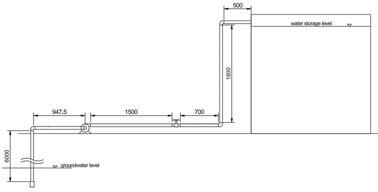
Example 1: Pump Operating Point for Pumping Groundwater to a Storage Tank
Groundwater at 25 °C will be pumped to a storage tank using 1½-inch Schedule 40 commercial steel pipe as shown in Figure 1.
A gate valve is installed for maintenance purposes and remains fully open during operation. A foot valve is installed at the suction line to maintain pump priming.
The elevation difference between the groundwater surface and the pipe outlet is 6.8 m.
A pump available locally has the following performance limits:
- Maximum head (shutoff head) = 100 m
- Maximum discharge (free delivery flow rate) = 25 L/s
Determine:
- (a) The operating flow rate and operating head when using 1½-inch Schedule 40 pipe.
- (b) The operating flow rate and operating head if 2½-inch Schedule 40 pipe is used instead.
Assume atmospheric pressure of 100 kPa.
Assumptions
- Dissolved solids in groundwater have negligible effect on fluid properties.
- Atmospheric pressure variation between suction and discharge is negligible.
System Head Equation
The system head is calculated using the mechanical energy balance:
Hsys = hz + hKE + hdP + hf
- hz = elevation head
- hKE = kinetic energy head
- hdP = pressure head
- hf = friction losses in pipes and fittings
The friction head is determined from:
hf = Ktotal v² / (2g)
Pump Characteristic Curve
The pump characteristic curve is estimated using the maximum head and maximum discharge:
Hpump = Hmax − aQ²
where
a = Hmax / Qmax²
Because the system curve uses m³/s for flow rate, the maximum pump discharge must be converted:
25 L/s = 0.025 m³/s
Therefore the pump characteristic curve becomes:
Hpump = 100 − 160000 Q²
Step-by-Step Calculator Procedure
-
Input elevation difference
6.8 m -
Select relative elevation:
Liquid source below discharge -
Elevation measured between:
source liquid surface and pipe outlet -
Pressure profile
Pressure 1 = 100000 Pa
Pressure 2 = 100000 Pa -
Pipe specification
- Pipe material: commercial steel
- Nominal pipe size: 1½ in
- Schedule: 40
- Total pipe length = 11.4475 m
-
Determine fluid properties
Using the Water & Steam Properties Calculator, select the TP input pair:- T = 298.15 K (25 °C)
- P = 0.1 MPa
- Density = 995.71 kg/m³
- Viscosity = 0.00085383 Pa·s
-
Add fittings
- Foot valve (1)
- 90° elbow (3)
- Gate valve fully open (1)
-
Input pump characteristic curve
Enter: 100 - 160000*Q*Q - Click Calculate Operating Point.
Note: Added fittings appear in the list below the schematic. They can be removed by clicking the “×” button.
Results
(a) Using 1½-inch Schedule 40 pipe:
- Operating flow rate = 0.0102 m³/s (10.2 L/s)
- Operating head = 83.31 m
(b) Using 2½-inch Schedule 40 pipe:
- Operating flow rate = 0.0182 m³/s (18.2 L/s)
- Operating head = 46.71 m
Engineering Insight
The operating point of a pump is determined by the intersection between the pump characteristic curve and the system head curve. Any change in the piping system will modify the system curve and therefore shift the operating point.
In this example, increasing the pipe diameter significantly reduces friction losses in the pipeline. As a result, the system curve shifts downward, allowing the pump to operate at a higher flow rate and lower operating head.
This behavior illustrates an important principle in pump system design: pipe friction losses strongly influence the operating point of a pumping system.
While larger pipe diameters reduce friction losses and increase the achievable flow rate, they also increase installation and material costs. Engineers must therefore balance hydraulic performance and economic considerations when selecting pipe sizes.
The optimal pipe size can be determined using the Optimum Pipe Diameter Calculator .
After determining the operating flow rate, engineers should also verify:
- Pump power requirement using the Pump Power Calculator
- Available suction head using the NPSH Available Calculator
These evaluations ensure that the selected pump operates efficiently without exceeding motor power limits or experiencing cavitation.
Common Pump Operating Point Searches
- How to find pump operating point?
- Pump curve and system curve intersection example
- Actual pump flow rate calculation
- System curve calculator with friction loss
- How pipe diameter affects pump performance?
This tool solves the intersection between:
Pump Head Curve H(Q) and System Head Curve H_system(Q)
System Curve, Pump Curve, and Operating Point Fundamentals
In pump-driven fluid systems, the actual flow rate and pressure are not determined by the pump alone, but by the interaction between the pump characteristics and the system resistance.
This interaction is described using two fundamental concepts:
- System Curve – represents how much head the system requires at different flow rates
- Pump Curve – represents how much head the pump can deliver at different flow rates
The point where these two curves intersect is called the operating point, which defines the actual flow rate and head of the system.
Traditionally, determining the operating point requires:
- Calculating system head over a range of flow rates
- Plotting system and pump curves
- Graphically identifying their intersection
This process can be time-consuming and often requires iterative calculations, especially when system conditions change.
This section explains the fundamental principles behind system curves, pump characteristic curves, and operating point analysis, which are essential for:
- Proper pump selection
- Energy-efficient system design
- Troubleshooting flow and pressure issues
- Optimizing piping and pump performance
By understanding these concepts, engineers can predict how a system will behave under different conditions and ensure reliable, efficient operation.
What is a System Curve?
The system curve represents the relationship between flow rate (Q) and the total head required by a piping system. It describes how much energy the system demands at different flow rates.
The system head includes:
- Static head (elevation difference)
- Friction loss in pipes
- Minor losses from fittings, valves, entrances, and exits
As flow rate increases, friction losses increase approximately with the square of velocity, causing the system curve to rise nonlinearly.
How is the System Curve Calculated?
Total system head is calculated as:
Total Head = Static Head + Friction Loss
For turbulent flow, friction loss follows:
Head Loss ∝ Q²
This quadratic relationship explains why small increases in flow rate can significantly increase required pump head.
What is a Pump Characteristic Curve?
A pump characteristic curve describes how a pump performs at different flow rates. The primary curve shows:
Head vs Flow Rate
Additional curves often include:
- Efficiency vs Flow
- Power vs Flow
- NPSH Required vs Flow
Each pump model has a unique characteristic curve determined by its design and operating conditions.
What Factors Affect Pump Characteristic Curves?
- Impeller diameter
- Rotational speed
- Impeller trimming
- Fluid density and viscosity
- Mechanical wear and internal clearances
Changing rotational speed shifts the curve according to the pump affinity laws:
- Flow ∝ Speed
- Head ∝ Speed²
- Power ∝ Speed³
What is the Pump Operating Point?
The operating point is the intersection between:
- The Pump Curve
- The System Curve
At this point:
Pump Head = System Required Head
This determines the actual discharge flow rate and operating head.
Why is the Operating Point Important?
The operating point determines:
- Actual flow rate delivered
- Energy consumption
- Pump efficiency
- Mechanical loading
- System stability
If the operating point is far from the pump’s Best Efficiency Point (BEP), energy consumption increases and mechanical stress rises.
What is the Best Efficiency Point (BEP)?
The Best Efficiency Point is the flow rate at which the pump operates with maximum hydraulic efficiency.
Operating near BEP:
- Reduces vibration
- Minimizes wear
- Improves energy efficiency
- Extends pump lifespan
What Happens if the System Curve Changes?
Changing system conditions shifts the operating point. Examples include:
- Valve throttling
- Pipe roughness changes
- Blockages
- Elevation changes
A higher system resistance shifts the operating point to lower flow rates and higher required head.
Can a Pump Deliver Any Flow Rate?
No. A pump cannot deliver a flow rate independent of the system. The actual flow rate is determined by the interaction between pump capability and system resistance.
How Does Pipe Diameter Affect the Operating Point?
Reducing pipe diameter increases friction loss, making the system curve steeper. This shifts the operating point to:
- Lower flow rate
- Higher head requirement
Increasing diameter flattens the system curve and increases achievable flow rate.
Why is Operating Point Analysis Important?
Understanding pump-system interaction ensures:
- Correct pump selection
- Energy-efficient operation
- Prevention of overload conditions
- Stable and predictable system performance
Proper operating point analysis is essential in water supply, industrial processing, HVAC systems, and irrigation networks.